San Diego Seismicity

A start-to-finish World Grids + Channels demonstration: a live USGS catalog pull becomes a georeferenced scene and a 66-year time replay of the San Diego region's earthquakes. Works flat or as a globe.

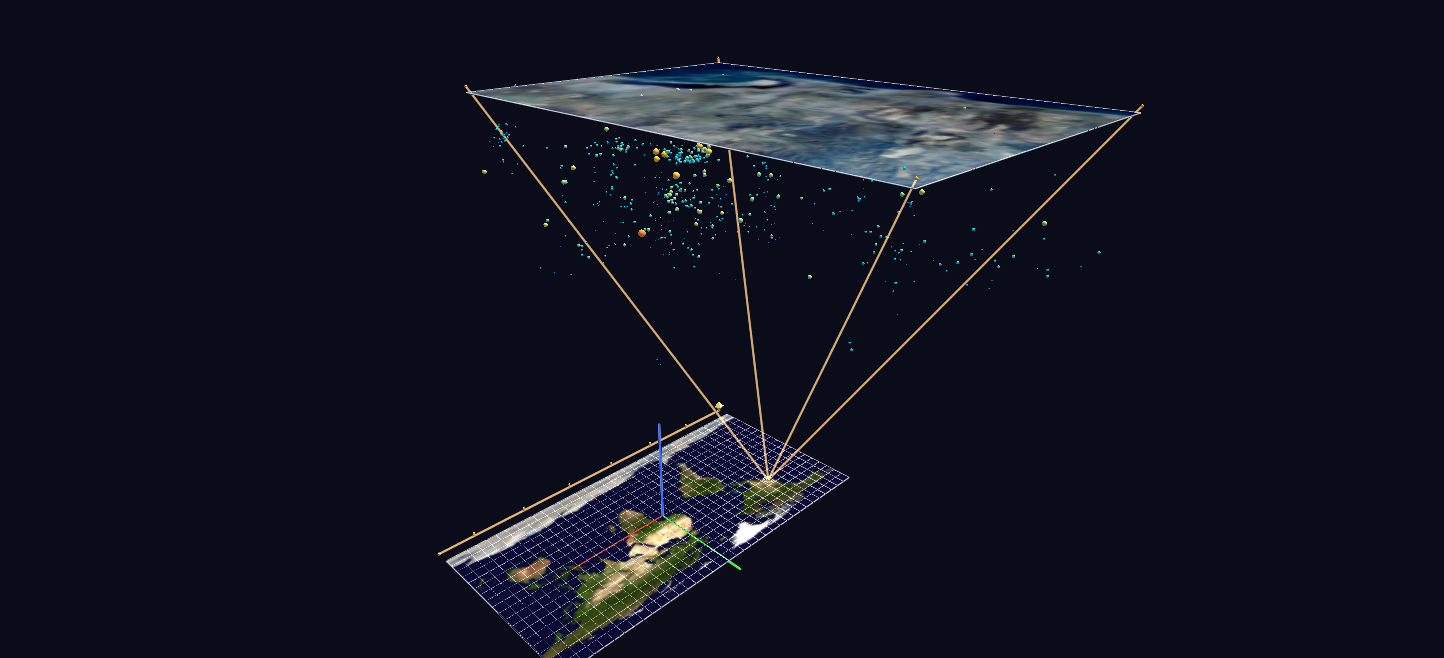
Try it: download this example below (or the full examples set), then open SD_Seismicity_Example/sd_quakes_gv_node.csv — or just drag its folder onto the GlyphViz window. Press Space to start the animation.

Download this example (7 MB)

What it is

The earthquakes of the San Diego region since 1960, 634 of them, shown the way a map inset shows a city: a small region blown up and lifted clear of the world map it came from, with lines joining the two. It is a worked example of two features working together, World Grids (maps that nodes attach to by longitude and latitude) and Channels (animation), and it runs from a live US Geological Survey (USGS) catalogue download to a finished, georeferenced scene.

Press Space and sixty-six years of seismicity replay in about 28 seconds.

What is on the screen

• The Earth. A Blue Marble world map lies flat at the origin, with a ten-degree graticule.
• The San Diego plate. An aerial mosaic of the region, around 191 by 280 units, hovers 230 units directly above its own footprint on the world map.
• The callout. On the world map, a glowing amber halo and a true-scale rectangle (four corner glyphs joined by four links) mark exactly the region the upper plate covers. Four more links rise from those corners to the plate's corners, a zoom frustum in true 3D, in the manner of a cartographic inset.
• The earthquakes. Each hypocentre is a sphere hanging beneath the aerial plate: its longitude and latitude are from the catalogue, and its depth hangs below the plate (exaggerated 6.5 times), so the seismicity volume fills the frustum under the photograph.

How to read an earthquake

Property	Encoding
Position	longitude and latitude from the catalogue; depth as distance below the plate
Size	magnitude, scaled quadratically, so large events stand out
Colour	magnitude, on a ramp from cold blue through cyan and gold to red
A label	every event of magnitude 3.5 or more has its label drawn on it
A link	every event carries a link to its USGS event page: select it and press U

Each event also has a colour index (1 to 20), so the = and − keys recolour a selection through a palette.

The replay

One animation frame is one calendar month, from about 1960 to the present (847 frames).

1. Every earthquake is born invisible.
2. In the month it happened it flashes to full brightness, then decays to a dim "memory" level. The bright glyphs are always the recent events; the dim field is the accumulated history.
3. In the final second of the loop, the whole catalogue relights to full brightness. Then the cycle restarts from an empty volume.
4. A timeline bar with decade ticks runs along the south edge of the world map, and a spinning amber cursor sweeps it. Its position is the current date.

Playback off, or Stop (Shift+Space), shows the complete static catalogue, because the Channels files only ever animate the scene's own values.

Things to try

• Orbit below the plate. The solid aerial plate blocks picking from above, so to select a hypocentre, orbit beneath or beside the plate, or switch the plate to wireframe.
• Turn either map into a globe. Press G to select a grid, and in the World Grid panel set Shape to Sphere. The Earth plate becomes a globe, and the events stay where they belong.
• Read the depth. Look from the side: the hypocentres form a volume under the photograph, so you can see how deep the events sit and where they cluster.
• Rebuild with a different threshold. --min-mag 1.0 hides the tiniest events; --start 1980-01-01 shortens the range.

How it is built

The scene is 665 nodes: two World Grids, the 634 hypocentres (children of the San Diego grid), the callout's corners and links, a timeline bar and its decade ticks. The replay is 847 frames over 316 Channels bindings. Only 315 channels animate 634 earthquakes, because every event born in the same calendar month shares one channel: one step-function opacity track per month. The timeline cursor is a translate_x channel, which works because channel values are coordinates in the node's own parent space.

The aerial mosaic carries no embedded location, so its extents (longitude −117.31 to −116.97, latitude 32.57 to 32.98) were solved by eye from four landmarks, with an estimated uncertainty of about 0.02 degrees. The generator, build_sd_quake_scene.py, does the whole pipeline: fetches the catalogue from the USGS service, builds and validates the scene, and snapshots the catalogue to data/usgs_catalog.csv so the scene can be rebuilt offline.

Source: USGS Earthquake Hazards Program catalogue (public domain). World map: NASA Blue Marble.