Vehicle Sales — Raw Auction Field

No aggregation. A seeded sample of 20,000 used-vehicle auction sales, one five-part glyph each — about 100,000 nodes, and a deliberate stress test at GlyphViz's practical node budget.

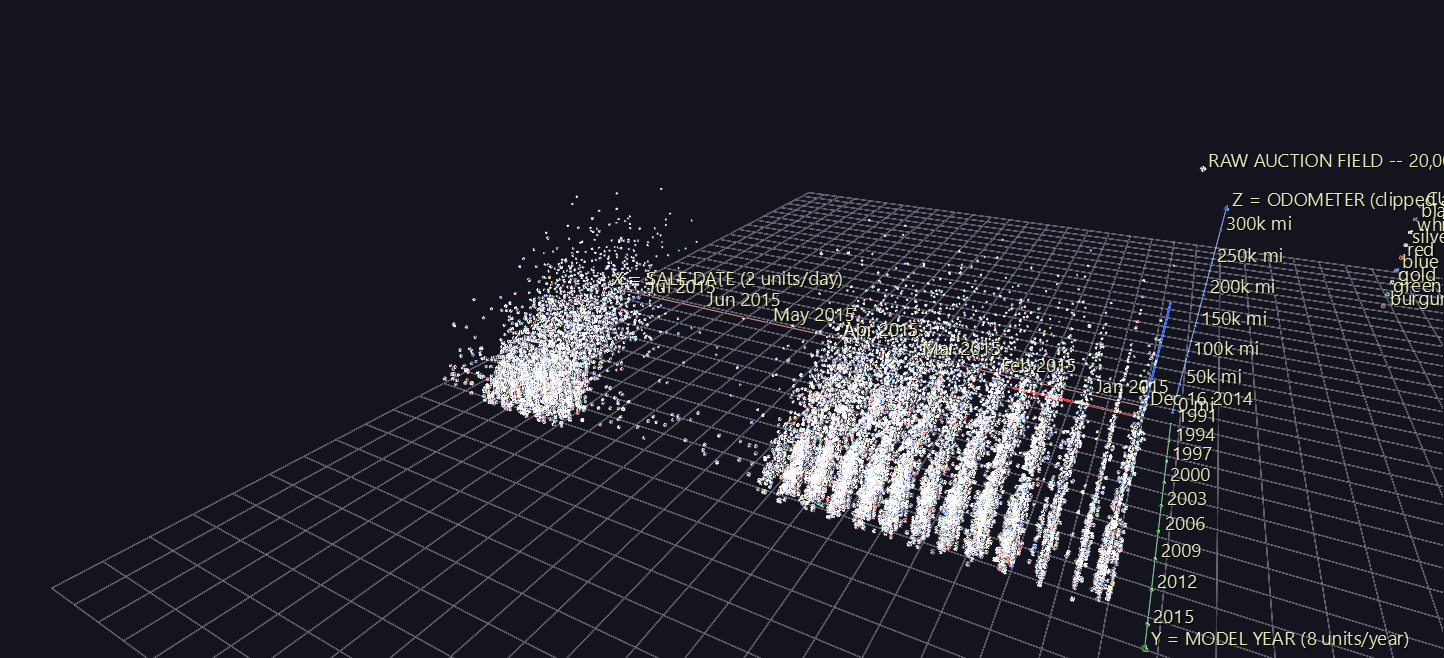
Two cities of glyphs: the December–March selling season and the May–June one, with April nearly empty between them. The vertical combs inside each are model years.

Try it: download this example below (or the full examples set), then open Vehicle_Sales_Example/Raw_Auction_Field/RawAuctionField_gv_node.csv — or just drag its folder onto the GlyphViz window.

Download this example (2 MB)

---

Reading one glyph

Every sale is one wire cube with four things mounted on it. The scene carries its own legend: an upright panel parked out at x = -395, clear of the data, so 100,000 glyphs don't render through its captions. Orbit left past the start of the time axis to find it.

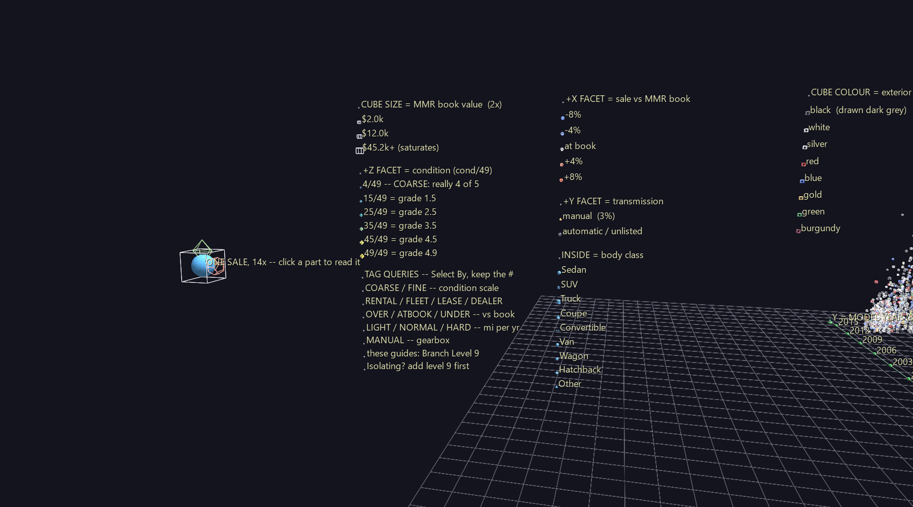
Part	Geometry	Encodes
the cube	wire cube, Cube topology	one auction sale. Colour is the exterior paint; size is the MMR wholesale book value (√-scaled, saturating at the 99th percentile ≈ $45k)
inside it	solid glyph at the cube's centre	body class by geometry — sedan = sphere, SUV = cube, truck = cylinder, coupe = cone, convertible = torus, van = dodecahedron, wagon = icosahedron, hatchback = octahedron. Coloured by the interior trim
+Z facet	wire octahedron	condition grade, exactly as the column publishes it: size and colour both run condition / 49, deep blue → teal → yellow
+X facet	wire dodecahedron	this sale against book — blue under MMR, near-white at it, red over
+Y facet	wire tetrahedron / sphere	transmission — gold tetrahedron for manual (about 3% of the lane), dim grey sphere for automatic

Paint names are mapped to RGB tuned for the black viewport, so a black car renders dark grey rather than invisible.

The axes

Three labelled rails stand outside the data box, coloured the way GlyphViz's own transform handles are — X red, Y green, Z blue.

Axis	Meaning	Scale
X	sale date	2 units/day, Dec 2014 → Jul 2015. Cars sharing a timestamp fan out +0.03 each, so a same-second auction batch of several hundred spreads instead of stacking
Y	model year	8 units/year, 1991 → 2015
Z	odometer	120 units at 300,000 miles, clipped

Tick labels are pinned with show_text, so they read without turning scene-wide tags on. The whole scaffolding — rails, ticks, legend — sits at branch level 9, which makes Select By → Branch Level → 9 pick it up in one click. That matters when you isolate a cohort: tick Add to current selection, then run your query, then Show Only Selected [I], and the axes stay under the glyphs you kept.

Querying the field

The Properties panel's Select By → Tag contains box is a case-insensitive substring match over tag text. Every one of a record's five nodes carries the same token string, so a query selects whole glyphs, not bare parent cubes.

Token	Selects	Share of the sample
#COARSE / #FINE	which of the two scales this row's condition column is on	12.0% / 88.0%
#RENTAL #FLEET #LEASE #DEALER	consignor class, read off the seller column	14.3% / 4.0% / 43.1% / 38.5%
#OVER #ATBOOK #UNDER	this sale vs MMR book, ±5% band	26.4% / 43.0% / 30.7%
#LIGHT #NORMAL #HARD	odometer per year of age: under 9k, 9–18k, over 18k	17.4% / 51.3% / 31.4%
#MANUAL	manual gearbox	3.0%

Keep the leading #. A bare OVER also matches every Land Rover.

---

Reverse-engineering a visualization

This scene was built first, straight off the raw columns, with no finding in mind. The analysis below came afterwards, run over all 558,837 rows of the source dataset. The tokens exist so that each result has a click path — so a claim you can only reach with pandas can be seen.

Two of the three results survive that test. The third is included because it doesn't, and knowing which is which is the point.

1. The condition column is two scales in one

The column's 41 distinct values are 1–5, 11–19, 21–29, 31–39, 41–49. There is no 6, no 7, no 8, no 9, no 10, and no multiple of ten anywhere. That is a fingerprint, not a distribution: the high values are a 1.1–4.9 grade stored ×10, and 64,853 rows store the same 1–5 grade rounded to an integer instead — 12.2% of the 531,258 sales that carry both a grade and an odometer reading.

Pooling the two scales does real damage to any analysis that touches condition:

	published column, pooled	rescaled to a common 1–5 grade
corr(condition, odometer)	−0.296	−0.528
R² of odometer ~ condition	0.088	0.279
corr(condition, price vs book)	0.218	0.278
β on condition in log(price) ~ log(mmr) + condition	+0.0049	+0.1099
R² of that model	0.9357	0.9409

log(mmr) alone gives R² = 0.9303, so reconciling the scales doubles what condition adds on top of the book value — and multiplies its coefficient by twenty-two. A notebook that regresses on condition as published is measuring a blend of two rulers.

And the scene was already drawing it. Because the +Z facet renders condition / 49 exactly as published, every coarse-scale row gets an octahedron about a tenth of the size and colour it has earned. In the sample, #COARSE rows draw at a median condition/49 of 0.061 when their true grade fraction is 0.600. Across the whole dataset 30,729 of them are graded 4 or 5 out of 5 — clean, low-mileage cars (median 22,585 miles, $17,950 book, one year old) wearing a wreck's badge.

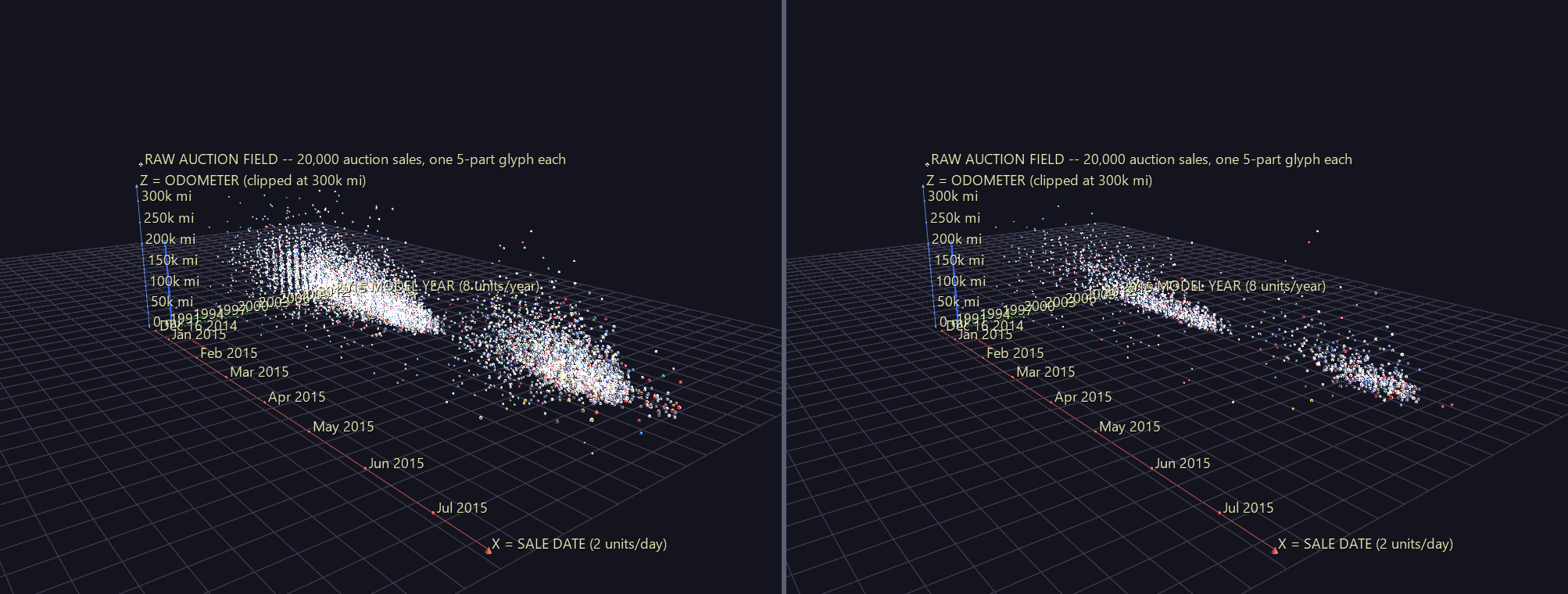
Select By → Tag contains → #COARSE → Show Only Selected. The full field (left) is a tall cloud reaching past 200,000 miles. The coarse-scale cohort (right) is a flat sheet along the floor: median model year 2012, median odometer 37,937 miles, median MMR $13,300. Genuinely low-graded cars — the 1,581 #FINE rows at grade ≤ 1.9 — sit where you'd expect instead: median 2006, 117,255 miles, $4,475.

Click any two of them and the point lands in one line:

The same car, twice. Upper: 2013 Lexus RX 350 Base, 36k miles, cond 44/49, sold $31.5k against a $30.2k book — a big yellow condition octahedron. Lower: 2013 Lexus RX 350 Base, 34k miles, cond 4/49, sold $32.3k against $31.1k — a speck of navy. Same model year, same mileage, same money, and the badge differs tenfold. The lower one was consigned by Lexus Financial Services, whose feed reports on the 1–5 scale.

Where it comes from. The artifact is per-consignor, not random. Seven sellers with 500+ sales report ≥90% of their cars on the coarse scale — GM Remarketing (98.5%), Enterprise Holdings/GDP (99.2%), Hertz/TRA (99.5%), Hertz Corporation/GDP (98.0%), PV Holding Inc/GDP (98.7%), Enterprise Vehicle Exchange/Tulsa (98.4%) and Ally (98.9%) — five of the seven being rental fleets, and 13,041 coarse rows between them. Across the whole dataset, #RENTAL consignors are 19.6% coarse against a 12.2% base rate, a 1.6× lift; the rest is spread thinly across mixed sellers. Query #COARSE, tick Add to current selection, query #RENTAL, and watch the overlap.

2. The book value is a precise number for new cars and a rough guess for old ones

MMR is a wholesale book estimate, and the residual (price − mmr) / mmr is nearly unbiased across most of the range. Its spread is not:

odometer	n	median residual	std dev	10th–90th percentile
< 25k	116,596	−0.3%	12.6	−10.8% … +7.6%
25–50k	150,061	0.0%	11.8	−10.6% … +9.1%
50–75k	83,362	0.0%	15.5	−14.0% … +13.4%
75–100k	61,760	0.0%	22.3	−23.8% … +22.0%
100–125k	49,188	−3.0%	25.9	−33.7% … +24.9%
125–150k	32,612	−5.1%	29.4	−40.1% … +27.9%
150–200k	29,052	−4.1%	36.5	−42.2% … +40.0%
> 200k	8,627	+4.0%	57.3	−41.4% … +75.0%

The residual's standard deviation grows 4.5× across the odometer range, and the 10–90 band widens from 18 points to 116. That is textbook heteroscedasticity, and it matters: an ordinary least-squares fit of price on MMR reports R² ≈ 0.98 and hides the fact that the book value is nearly uninformative at the top of the mileage axis.

Since the odometer is the Z axis here, that shows up as height.

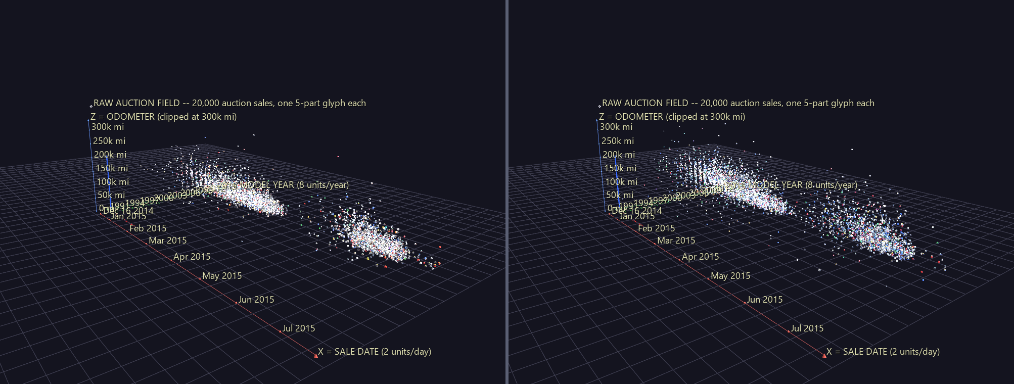
Left, #ATBOOK — sales within ±5% of book — is a low dense slab, median odometer 36,533 miles. Right, #UNDER climbs: median 73,114 miles. #OVER behaves the same way (median 68,069). Both tails live up high; the agreement lives down low.

3. The one the picture will not show you

The market has a real seasonal lift. Comparing each sale only against its own make × model × year × grade cell (cells of 20+ sales, so the mix can't move the answer), the median residual climbs steadily through tax-refund season and resets:

	Dec 2014	Jan	Feb	Mar	May	Jun	Jul 2015
median like-for-like residual	−0.31%	−0.24%	+0.23%	+0.62%	−0.69%	+0.17%	+0.48%

In the sample that means the #UNDER share falls monotonically from 35.9% of December's sales to 27.5% of March's. It is a genuine, robust result — and isolating #UNDER shows you essentially nothing, because an eight-point change in the density of a scattered cohort along a 420-unit axis is not something eyes read.

That is worth stating plainly. Selection filtering turns a scene into an instrument for categorical structure and spatial arrangement — where a cohort sits, how tall it stands, what shape it takes. It is not an instrument for conditional rates. GlyphViz will select the cohort and tell you how many nodes are in it; it will not tell you what fraction of a slab that is. When the answer is a ratio that changes slowly along an axis, go back to pandas.

---

Structure

branch level 9   83 nodes: 3 axis rails (Link nodes), 28 pinned axis
                 labels, 3 legend columns, and an assembled 14x glyph
branch level 0   the car          wire cube, Cube topology, paint colour,
                                  sized by MMR
branch level 1   ├─ interior      solid body-class glyph, translate_z = -1
                 │                (zeroes the Cube placement distance)
                 ├─ +Z facet      condition octahedron
                 ├─ +X facet      deal dodecahedron
                 └─ +Y facet      transmission tetra / sphere

Facet children mount with translate_z = −(1 − 1/√3), because Cube topology places a child at base_radius + tz along the face normal while the cube's rendered half-extent is 1/√3 — that pulls each child's centre back onto the face plane. Verified against compute_world_positions on sampled glyphs.

Regenerate with examples/Vehicle_Sales_Example/generate_vehicle_sales_example.py; --raw-rows and --seed control the sample.

Honest caveats

The scene renders the column as published, artifact and all. That is the point — it is the raw auction field — but it does mean the +Z facet is wrong for 12% of the glyphs, in a specific and now-documented way. Each of those cars' condition facet says so in its own tag text.

The consignor classes are a keyword heuristic over a free-text seller column with thousands of spellings. #RENTAL, #FLEET, #LEASE and #DEALER are good enough to make the mechanism selectable; they are not an audit of the auction industry. #DEALER in particular is a residual bucket.

About 205 records are timestamped Jan–Feb 2014, ten months before the real auction window, and are dropped — they stretched the time axis 2.5× for nothing. The April 2015 gap you can see in the field is not that: it is real, and the handful of April sales that do exist behave strangely (median 16% under book across the full dataset).

Miles per year uses age clipped at one year, so #HARD is a floor on use intensity rather than an exact rate for current-model-year cars.

Performance is the honest cost of the design. 100,000 nodes at 1280×720 clocks around 300 ms/frame headless. Interactive is better, but this scene is meant to push the renderer. With 20,000 tags, turning all labels on is brutal — the default (labels on selection only) is the way to inspect individual cars.

Data

Kaggle, syedanwarafridi/vehicle-sales-data — 558,837 US wholesale auction records (Dec 2014 – Jul 2015) with make, model, trim, body, transmission, VIN, state, condition, odometer, colour, interior, seller, MMR book value, selling price and sale date. The two aggregate scenes built from the same file are Market Galaxy and Depreciation Grid.