Importing point clouds (LIDAR)

Meshes ▸ Import Point Cloud…, or drag a .las/.laz/.xyz/.pts file onto the window.

GlyphViz reads LIDAR and scan data into a Point Cloud topology node: one parent glyph you can move, rotate and scale, with one real node per point underneath. Those points are not a special kind of object — they are ordinary nodes that happen to draw as a batch, so every one of them is clickable, labellable, Channels-bindable, and saves into the scene CSV like anything else.

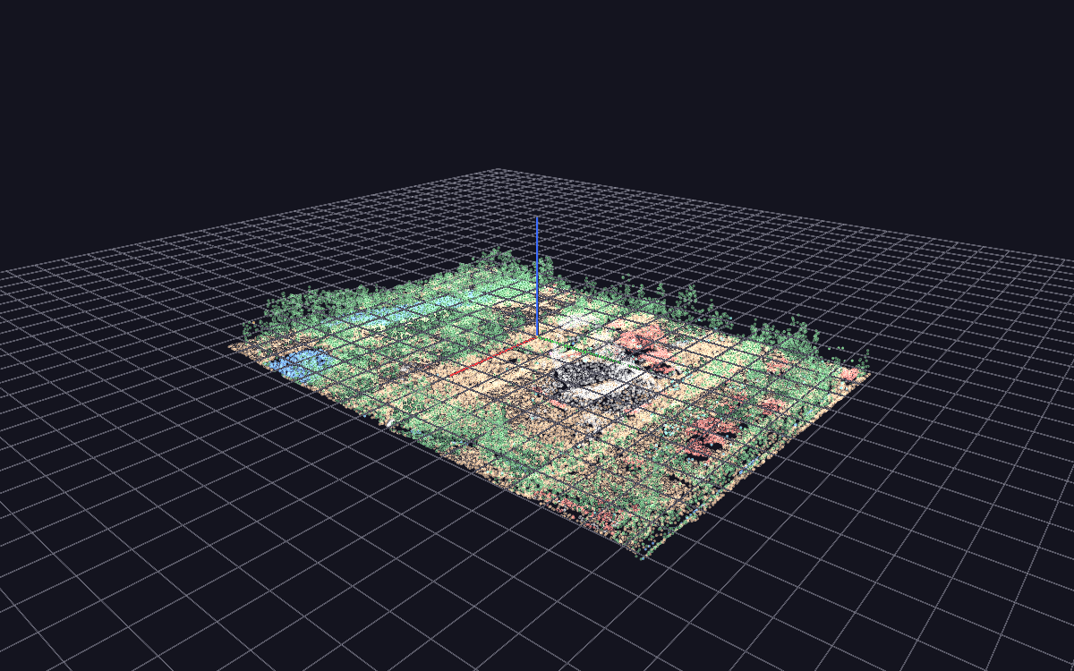
The formats, and why they are all open

LAS is binary, but it is not proprietary. It is a published ASPRS specification — the spec itself lives at github.com/ASPRSorg/LAS — and LAZ, its lossless compressed form, became an OGC Community Standard in September 2026.

Extension	What it is	Read by
.las	ASPRS LAS 1.0–1.4, the LIDAR interchange format	laspy
.laz	LAZ — LAS losslessly compressed to 7–20% of its size	laspy + lazrs
.ply	Stanford PLY, point-only or a mesh's vertices	trimesh
.xyz .pts .txt .csv	ASCII x y z [r g b], comma or whitespace	built in

A dropped .ply still goes to the mesh importer, as it always has — a dropped PLY is far more often a model than a scan. Use Import Point Cloud… explicitly to bring one in as points. .csv and .txt are likewise only offered through the file dialog, because a dropped CSV is a scene.

E57 is not supported. It is an open ASTM standard, but reading it needs a native library GlyphViz does not bundle; convert to LAS or PLY first.

What the dialog shows you before you commit

Opening a file reads its header first and reports what is actually in it — point count, extent in source units, and which of RGB, classification and intensity it carries. On a LAS or LAZ file that is nearly free however large the file is, because those facts live in the header.

That report exists because every one of those facts changes what a sensible import looks like. A 10-million-point tile in State Plane feet with no RGB needs different answers than a 200,000-point coloured scan in metres.

Keep at most

How many points to import. 100,000 is the comfortable default, and there is no upper limit — type a number at or above the file's own point count and every point in it is imported. The field is a suggestion about what you want, not a ceiling on what GlyphViz will accept.

The renderer is not what limits this — it draws a million points in 0.63 ms per frame, and a 442,767-point import runs at about 400 fps. The node model is: every point is a real node, costing about 2 KB of memory and about 90 bytes in the saved scene file.

Points	Import from LAZ	Saved scene	Save	Reopen	Memory
100,000	1.4 s	9.1 MB	1.0 s	1.4 s	~200 MB
442,767	4.0 s	40.7 MB	4.2 s	6.3 s	~900 MB

Scenes saved before September 2026 are much larger

GlyphViz used to save every node as a full 94-column ANTz-compatible row, about 550 bytes a point — that made the 442,767-point scan a 243 MB file that took 15 s to save. It now writes only the columns a scene uses. Opening one of those older scenes and saving it shrinks it in place.

Importing is much cheaper than saving. Bringing a large cloud in and flying around it is comfortable well past the default; it is keeping it as a scene file that gets expensive.

Method

How the points to keep are chosen.

• Random sample (default) — unbiased and reproducible. The same file and the same settings give the same cloud every time.
• Voxel grid — one point per occupied cell of a 3-D grid, so density is evened out instead of inheriting the scanner's. Measured on a real 10.6-million-point tile decimated to 100,000: voxel reaches 85% of the cells the full cloud occupies where random reaches 74%, at half the density spread. Because the grid is volumetric it moves points off flat ground and onto structure — trees, buildings — which is usually what you want to look at. Takes about twice as long.
• Every Nth point — fastest, and exactly reproducible without a random seed. Be careful with it: a file written in acquisition order has its rows grouped by flight line, so a stride can beat against the scan pattern and sample stripes rather than the scene.

Colour by

Automatic takes the file's own RGB when it has any, then classification when the file is genuinely classified, then an elevation ramp. Most public LIDAR has no RGB at all, so the other two are what usually make a scan readable rather than being fallbacks.

• File RGB — 16-bit or 8-bit is detected from the data, not assumed.
• Classification — ASPRS codes in the colours every LIDAR tool draws: ground brown, vegetation green by height, buildings red, water blue. Codes past the standard 0–18 table (LAS 1.4 reserves 64+ for user definition) get distinct generated hues.
• Elevation — a blue→green→warm-white ramp over height.
• Intensity — return strength, dark to bright.

Both ramps normalise over the 2nd–98th percentile rather than min/max, because a handful of noise returns at the top of the range would otherwise squeeze every real value into the bottom of the ramp.

Point size

The rendered size of every point, in pixels. Stored on the cloud's parent as ratio = size / 20, so you can change it afterwards from the Properties panel's Ratio field. One size per cloud — fixed-function OpenGL has no per-point size. To encode a second variable, use colour, or split the scan across several cloud parents.

Fit to width

The world-space width the scan is scaled to, measured across its larger horizontal axis. 360 is GlyphViz's own 1:1 frame — the width of a default World Grid, and a full sweep of longitude — so an imported scan lands at the same scale as everything else and can be dropped onto a grid without retuning.

This matters more than it sounds. A georeferenced tile arrives in CRS units with an enormous origin: the Autzen Stadium test file runs 635,577 to 639,003 easting in Oregon State Plane feet. Imported raw it would be a speck 800,000 units from the origin.

The scale is uniform across all three axes and derived from the horizontal extent only, so the scan is never stretched. Centre and scale are measured from the 0.1–99.9 percentile box rather than the raw bounding box: airborne LIDAR reliably contains a few gross outliers (birds, cloud returns), and one point a kilometre up would otherwise shrink the whole scan toward invisibility.

Vertical exaggeration

Multiplies Z alone. 1.0 is truthful and is the default. Terrain work routinely uses 2–3×, because 200 m of relief spread over 4 km reads as flat otherwise — but it is a distortion, which is why it is opt-in.

Keep classifications

Import only the ticked classes. Dropping Ground (class 2) is the usual first move on an aerial tile: it is most of the points, and removing it reveals the buildings and canopy underneath.

The filter runs before the decimation, so your point budget is spent on the classes you asked for. Ask for 100,000 points and drop ground on a tile that is 70% ground, and you get 100,000 non-ground points — not 30,000.

After the import

The cloud is merged into the loaded scene rather than replacing it, with ids rebased exactly as File ▸ Merge does. A scan is nearly always context for something else — sensors placed inside a building, per-tree glyphs over a canopy — so replacing your scene would be the wrong default.

The cloud's parent node carries the provenance in its label: how many points, how they were coloured, what they were sampled from, which classes were kept, and any exaggeration applied. That label is the only record of how the cloud was made, since a saved scene has no other memory of it. The points themselves carry no labels, deliberately — see the topology reference.

From there it is an ordinary GlyphViz scene:

• Move, rotate, scale the parent and the whole cloud follows.
• Click a point to select it; it is a real node with an id, and the Properties panel edits it.
• Label the handful that matter with show_text, or by selecting them.
• Save with Ctrl+S — the cloud travels in the node CSV with no new column and no external file.
• Parent other nodes to the cloud's parent to place glyphs in the scan's own coordinate frame.
• Retune the whole scan with the parent's Topo Scale, which multiplies all three axes.